Audio Feature Surfing
Feature Perceptualisation Challenges
Perceptualising audio features for working with big audio data
Across arts, humanities and sciences, researchers are recording and collecting repositories of audio archives well beyond listenable compass. Whilst we can in theory apply machine listening and learning methods to search for salient patterns in, and make sense of this big audio data, much is lost in not being able to engage perceptually with the raw audio. We need new ways to ‘get to know’ audio archives, other than through remote statistical probing for many reasons: to verify data integrity (is it blank, is it distorted etc), to aid cataloging and search (is it music, spoken or environmental recording?) or in scientific domains, to help interpret the models we build from it.
One approach, already being explored in the context of soundscape ecology, is the false-colour spectrogram. Soundscape ecology is a rapidly growing field in which the potential for acoustic analyses to address previously hard-to-reach questions is being explored. Researchers globally are amassing vast audio archives using remote, schedulable devices to record terabytes of environmental soundscapes. Patterns of ecological interest often occur over weeks, months, or even years, involving many terabytes of data, only a fraction of which can ever be listened to.
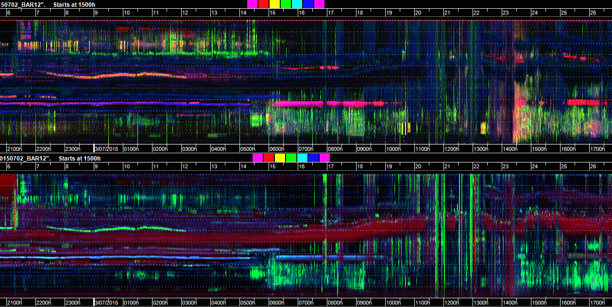
Michael Towsey’s group in QUT have been experimenting with false-colour spectrograms for visualisation of long-form recordings1.These are essentially visualisations of audio features, calculated on short audio recordings (typically 1 minute). Three indices known to capture distinct characteristics (ie orthogonal) are mapped to RGB values and displayed in spectrogram-like format, enabling spectro-temporal info over full days to be viewed at a glance (Fig 1)
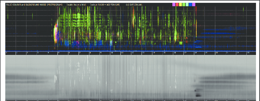 Fig 1. Example of a false-colour spectrogram from Towsey et al 2014. This is derived from a combination of normalized spectrograms for ACI, 1-H[t] and CVR. The vertical gridlines are at one hour intervals, starting and ending at midnight. The horizontal gridlines are at 1 kHz intervals.
By calculating the indices over full frequency range and representing three indices as RGB pixels values, diurnal patterns of weeks and months, even years can be viewed, in an “Extended Acoustic Summary Image” (Fig 2)
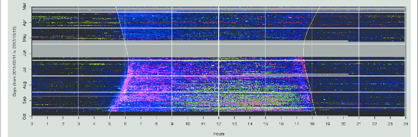 Fig 2. Example of a Extended Acoustic Image from Towsey et al 2014. An Extended Acoustic Summary image for the months March to October, 2013 Each pixel RGB value represents values for three acoustic indices for a 1 minute recording
The false-colour spectrogram will be as informative as the indices it is generated from – and this will vary task to task. This approach is promising for time-series data from a single point, but many other possibilities exist, including interactive resynthesis of audio features, for example.
Challenge
(How) can feature visualisation – or sonification/ resythnesis – provide a meaningful perceptual summary of large audio archives? Can ecologically relevant features be distinguished - such as animal sounds (biophony), weather (geophony) and machinery (technophony)? Can silent and distorted files be made apparent? Might interactive perceptualisation afford deeper insights?
Data
Two 3 hour dawn chorus recordings are available, made in different habitats at the same time. Each is segmented into 180 one minute mono wav files. The recordings start 90mins before sunrise, capturing the onset of the dawn chorus. Beside a bird chorus of increasing density, there are some sheep, various engines (planes, cars) and a thunder storm, followed by rain.
UK dawn chorus recordings on Fig Share
Audio features for gender-based conversational dynamics.
One of the many excruciating features of Trump’s presidential election campaign was his constant interruptions of Hilary Clinton during the presidential debate. And recent research published in the Journal of Social Sciences2 reveals similar gender differences in interruptions in academic job talks. Automatic analysis of speaker characteristics, such as gender, would be a powerful tool in analysis of conversational dynamics in oral history, gender studies and numerous other humanities disciplines.
Challenge
Could machine listening in combination with supervised learning, or even unsupervised clustering be used to discriminate between voices in an interview in order to identify conversational dynamics?
Participants are invited to consider which audio features and/or machine learning methods might be best applied.
Trump vs Clinton Presidential Election Campaign 2016.
Data.
For exploration, an audio file of Trump’s Clinton interjections is available here
Resources/ Links
CataRT
Standalone: http://forumnet.ircam.fr/product/catart-standalone-en/
False Colour Spectrogram Sketch
Python implementation of Acoustic Indices for soundscape analysis https://github.com/sandoval31/Acoustic_Indices
Principle Latent Component Relationships
Memory Mosaic
App on Appstore
Video on Vimeo
Daphne Oram Browser
Video on Vimeo
Towsey, Michael, Liang Zhang, Mark Cottman-Fields, Jason Wimmer, Jinglan Zhang, and Paul Roe. “Visualization of long-duration acoustic recordings of the environment.” Procedia Computer Science 29 (2014): 703-712. ↩
Blair-Loy, Mary, Laura E. Rogers, Daniela Glaser, Y. L. Wong, Danielle Abraham, and Pamela C. Cosman. “Gender in Engineering Departments: Are There Gender Differences in Interruptions of Academic Job Talks?.” Social Sciences 6, no. 1 (2017): 29. ↩
CHALLENGES
info